-
[Matplotlib]파이썬 기본 데이터 시각화파이썬 머신러닝 2023. 12. 24. 22:15
Matplotlib — Visualization with Python
seaborn seaborn is a high level interface for drawing statistical graphics with Matplotlib. It aims to make visualization a central part of exploring and understanding complex datasets. statistical data visualization Cartopy Cartopy is a Python package des
matplotlib.org
어떤 프로그래밍언어나 프로그램을 사용하든 데이터를 다루는 작업(통계, 수치해석, 머신러닝 등)의 결과를 보기 위해선 시각화가 필요하다. 그래프로 데이터의 전체적인 경향을 보지않고 작업을 할 수는 없으며, 결과를 보기위해서라도 시각화가 필요하다. 즉 시작하기에 앞서 시각화 툴이 손에 익어야 한다는 것이다. 예쁘게 시각화를 하고자 하면, maplotlib보다 seaborn을 사용하는게 좋겠지만, 최종본이 아닌 이상 그럴필요는 없으니 maplotlib으로도 충분하며, maplotlib를 warping한 seaborn 특성상 matplotlib와 함께 사용해야만 한다. 따라서 이번에는 matplot의 기본적인 사용법을 소개하고자 한다. (참고로 MATLAB과 비슷한 문법을 사용하니 MATLAB에 익숙하다면 matplotlib도 쉽게 사용할 수 있을 것이다.) 모든 기능을 소개할 수는 없고, 개인적인 경험을 기반으로 자주 사용하는 것을 정리하였다.
추가적으로 matplotlib에 대해서 설명하면서 엑셀로 하면 안되냐는 말을 들은 적이 있다. 물론 사용하지 못할 것은 없지만, 데이터의 갯수가 수천에서 수백만개가 되는데 어느 세월에 처리한 데이터를 csv로 내보내며, 그 많은 데이터를 어떻게 드레그해서 그래프를 그릴까? 많은 데이터를 다룰 때 엑셀같은 GUI 프로그램은 렉이 걸리기 때문에 고사양의 컴퓨터가 필요하며, 파이썬에서 처리한 데이터를 파이썬에서 직접 그래프 그리는 것보다 훨씬 그레프 그리는데 오래걸릴 것이다. 처음 배우는 입장에서는 코드가 익숙지 않겠지만, 조금 시간이 지난다면 GUI로 하나하나 클릭하는 것이 더욱 귀찮게 여겨질 것이다.
0.설치
cmd, PowerShell, git console 등 command line에 아래와 같이 입력한다.
pip install matplotlib #만약 numpy, pandas가 설치되어 있지 않다면 같이 설치할 것만약에 pip를 찾을 수 없다. pip가 명령어, 프로그램 등이 아니다라고 한다면, 환경변수에 pip가 등록되지 않은 것이니 아래 링크를 참고하면 된다.
https://sidreco.tistory.com/14
파이썬 + VScode 머신러링 환경 구축
아나콘다 + jupyter notebook이나 google colab 등이 있지만, 아나콘다는 쓸대없이 무겁고, colab은 데이터 파일 올리기가 귀찮다. 필자는 직접 파이썬을 설치하여 pip로 필요한 패키지만 설치하는 것을 선
sidreco.tistory.com
1.Import, 한글 설정
import numpy as np
import pandas as pd #데이터를 읽어들이는데 필요
import matplotlib.pyplot as plt

#한글 폰트 설정
plt.rcParams["font.family"] = "Malgun Gothic" #plt.rc("font", family="Malgun Gothic")으로 해도 됨
plt.rcParams["axes.unicode_minus"] = False #-부호 깨짐 방지

#한셀에 여러 출력이 나오도록 설정(선택)
from IPython.core.interactiveshell import InteractiveShell
InteractiveShell.ast_node_interactivity="all"
1.1 설치된 폰트 리스트 확인하기
#설치된 폰트 이름 확인
import matplotlib.font_manager as fm
font_list = [font.name for font in fm.fontManager.ttflist]
font_list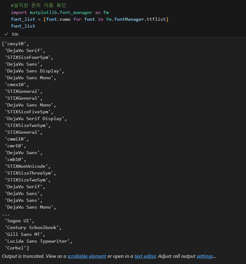
1.2 폰트 추가하기
Malgun Ghothic을 사용해도 한글 출력에는 문제가 없지만 예쁜 그래프를 위해 다른 폰트를 사용하고 싶을 수도 있다. 또한 NanumGothic을 비롯하여 윈도우에 설치가 되었지만, 폰트 리스트에 보이지 않는 폰트가 있다. 이러한 폰트들은 수동으로 추가해주어야 한다.( 그래프 한글 출력에는 문제가 없지만 , 폰트 리스트를 살펴보면 Malgun Gothic이 세개나 있는데, 왜 이런지 댓글로 알려주면 감사하겠습니다.)
#폰트 리스트에 없는 폰트 추가 방법
import matplotlib.font_manager as fm
fontpath = "C:/Windows/Fonts/NanumGothic.ttf"
fm.FontManager.addfont(fm.fontManager, path=fontpath) #matplotlib.font_manager.fontManager.ttflist에 폰트 추가
fm.FontProperties(fname=fontpath, size=12) #해당 폰트의 properties 추가, size 옵션으로 기본 폰트 크기 설정
plt.rc("font", family="NanumGothic")
2.공통적으로 적용되는 함수
2.1 figure, show, savefig, title, xlabel, ylabel, xlim, ylim
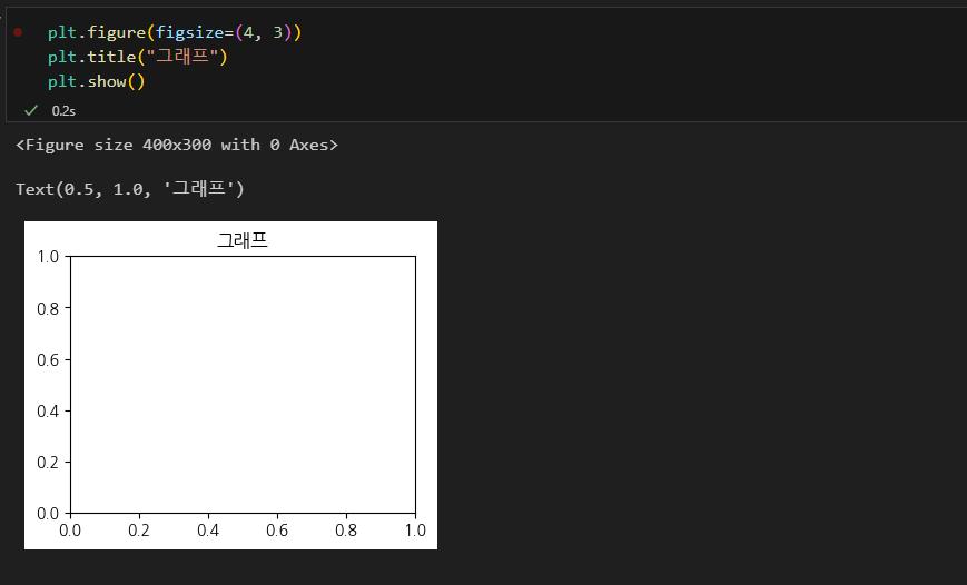
plt.figure() #빈 이미지 생성
plt.figure(dpi=100) #dot per inche로 그래프 해상도 조절 가능
plt.figure(figsize=(4, 3)) #figsize 키워드로 그래프 가로, 세로 크기 설정(단위 inche)

plt.show() #그래프 보여줌

plt.savefig("파일 이름", format="png", bbox_inches="tight")
#bbox_inches:boundary_box_inches, 그래프 여백을 어떻게 할지 정하는 옵션
plt.savefig("파일 이름", format="png", bbox_inches="tight", pad_inches=3)
#bbox_inches="tight"일 때 pad_inches 옵션을 주어 여백을 조절할 수 있다.

plt.title("그래프 제목", size=15) #size 옵션으로 폰트 크기 설정 가능
plt.xlabel("x축") #x축 라벨
plt.ylabel("y축") #y축 라벨

plt.xlim(left=1, right=3) #x축 범위 수동 설정(안하면 데이터 범위에 맞춰서 자동으로 조절됨)
plt.ylim(bottom=0.5, top=1) #y축 범위 수동 설정(안하면 데이터 범위에 맞춰서 자동으로 조절됨)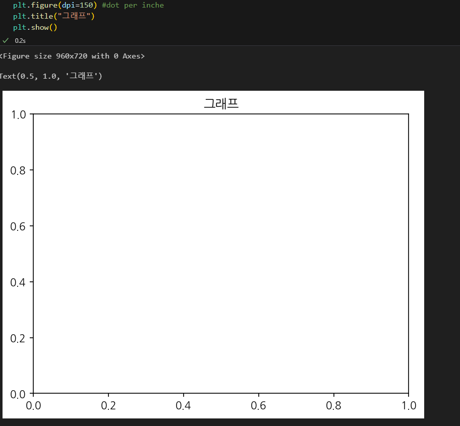

bbox_intches="tight" 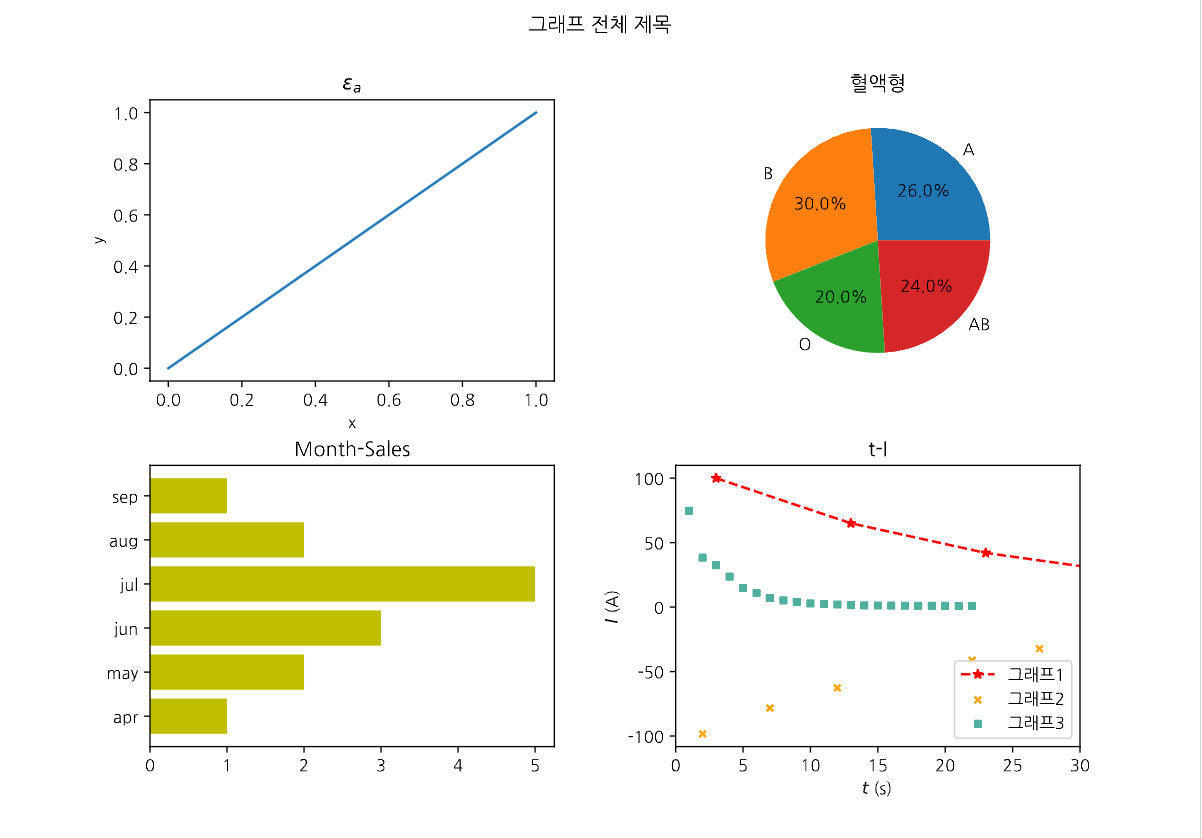
기본 옵션 
bbox_inches="tight", pad_inches=5 2.2 legend() -범례 생성
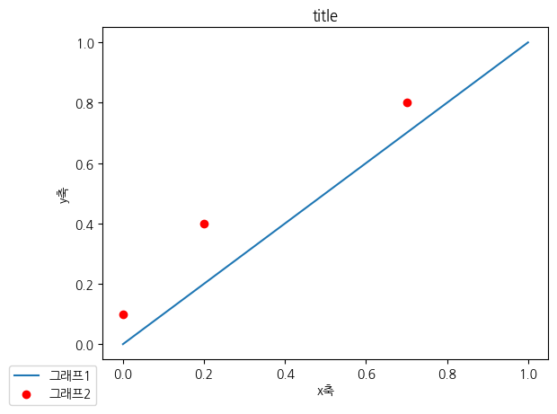
#legend
plt.figure(dpi=100)
plt.title("title")
plt.xlabel("x축")
plt.ylabel("y축")
plt.plot([0, 1], [0, 1], label="그래프1")
plt.scatter([0, 0.2, 0.7], [0.1, 0.4, 0.8], label="그래프2", color="r")
plt.legend() #옵션을 주지 않으면 알아서 최적 위치로 설정
plt.show()

#범례 위치 조절하기
plt.legend(loc="옵션")
#사용가능한 옵션
#'best', 'upper right', 'upper left', 'lower left', 'lower right', 'right',
#'center left', 'center right', 'lower center', 'upper center', 'center'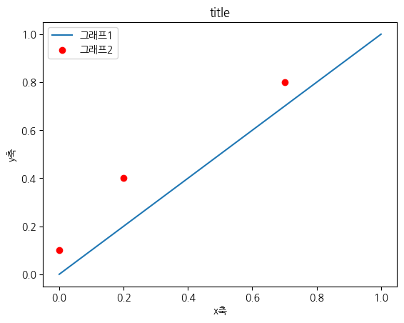
#범례 위치 조절하기 2
plt.figure(dpi=100)
plt.title("title")
plt.xlabel("x축")
plt.ylabel("y축")
plt.plot([0, 1], [0, 1], label="그래프1")
plt.scatter([0, 0.2, 0.7], [0.1, 0.4, 0.8], label="그래프2", color="r")
plt.legend(bbox_to_anchor=(1.25, 0.5)) #boundary_to_anchor
plt.show()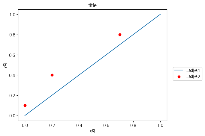
bbox_to_anchor=(0, 0) 3.pandas로 데이터 읽어들이기
df = pd.read_csv("csv 파일 경로")
#만약 인코딩이 달라 문제가 생기는 경우 아래처럼 해결
df = pd.read_csv("csv 파일 경로", encoding="utf-8") #이것도 안되면 euc-kr로 해보기
#파일에 한글에 있는데 인코딩이 utf-8이나 euc-kr이 아닌 경우 오류가 발생할 수 있음
read_excel 함수도 있지만 추천하진 않는다.(특히 한 엑셀파일에 여러 sheet가 있을 경우) 엑셀에서 csv으로 내보내서 처리하는 것을 추천한다. 참고로 csv는 Comma-Seperated Value의 약자이다.
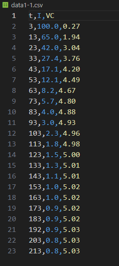
csv파일 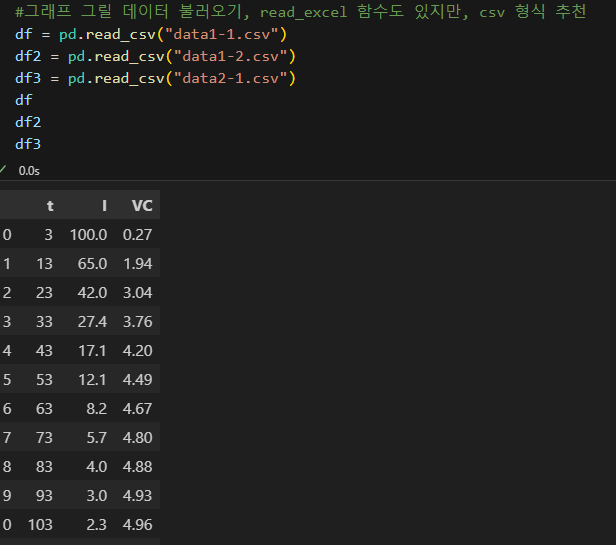
4.Scatter
#scatter
plt.figure(dpi=150)
plt.title("$\mathbf{t-I}$") #$로 둘러서 title, xlabel, ylabel에 latex 문법 사용가능, legend에는 불가능
plt.xlabel("$t$ (s)")
plt.ylabel("$I$ (A)")
plt.scatter(df["t"], df["I"], label="그래프1", s=7, color='r') #color 옵션을 주지 않으면 기본은 파란색
plt.scatter(df2["t"], df2["I"], label="그래프2", s=7, color="orange") #color 옵션에 CSS 색상코드 사용할 수 있음
plt.scatter(df3["t"], df3["I"], label="그래프3", s=7, color="#50df9e") #color 옵션에 헥스코드 사용할 수 있음

plt.xlim(left=0, right=50)
plt.legend() #그래프 모두 그린 다음 입력해야 범례가 모두 표시됨
plt.show()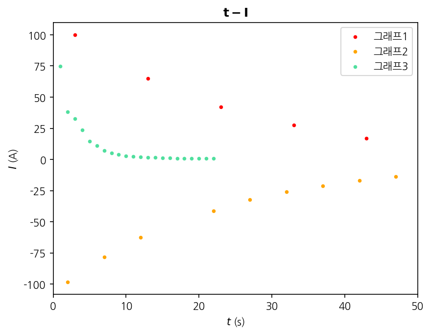
Marker 옵션
plt.figure(dpi=150)
plt.title("t-I")
plt.xlabel("$t$ (s)")
plt.ylabel("$I$ (A)")
#여러가지 마커옵션, 종류는 공식 문서를 참고할 것
plt.scatter(df["t"], df["I"], label="그래프1", s=15, color="#50af9e", marker='*')
plt.scatter(df2["t"], df2["I"], label="그래프2", s=15, color="#50af9e", marker='x')
plt.scatter(df3["t"], df3["I"], label="그래프3", s=15, color="#50af9e", marker='s')

plt.xlim(left=0, right=50)
plt.legend() #그래프 모두 그린 다음 입력해야 범례가 모두 표시됨
plt.show()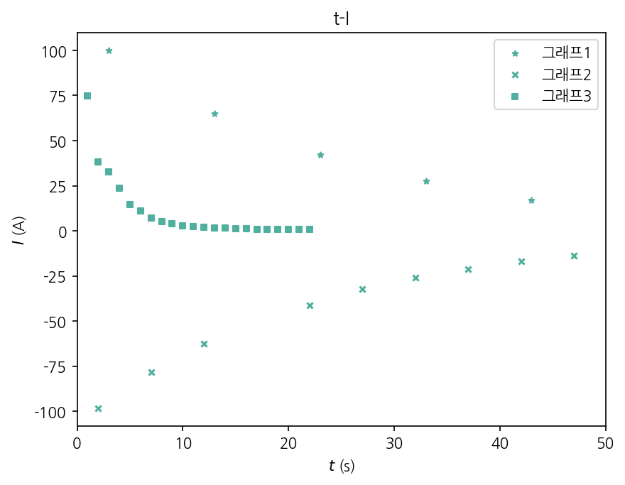
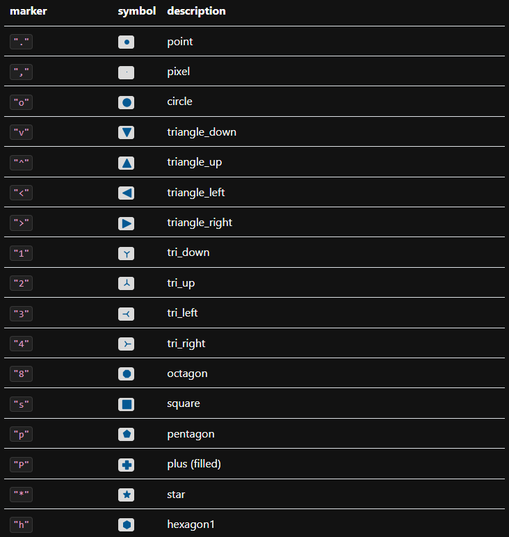
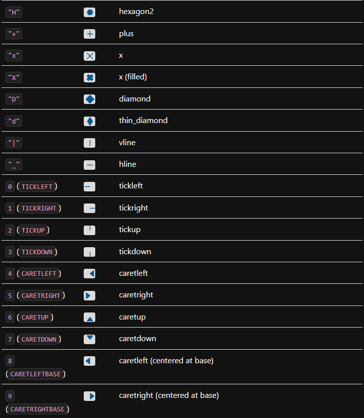
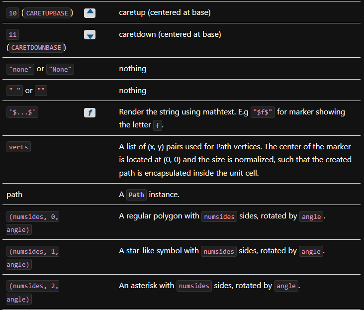
https://matplotlib.org/stable/api/markers_api.html
matplotlib.markers — Matplotlib 3.8.2 documentation
matplotlib.markers Functions to handle markers; used by the marker functionality of plot, scatter, and errorbar. All possible markers are defined here: marker symbol description "." point "," pixel "o" circle "v" triangle_down "^" triangle_up "<" triangle_
matplotlib.org
공식 문서에서 마커 종류를 살펴보면 다음과 같다.
5.plot
x, y 점들을 입력해주면 점들을 직선으로 이어준다.
#plot -점들을 직선으로 이어줌
plt.figure(dpi=150)
plt.title("t-I")
plt.xlabel("$t$ (s)")
plt.ylabel("$I$ (A)")
plt.plot(df["t"], df["I"], label="그래프1") #x데이터, y데이터

plt.xlim(left=0, right=50)
plt.legend() #그래프 모두 그린 다음 입력해야 범례가 모두 표시됨
plt.show()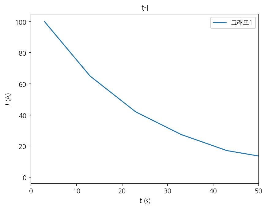
5.1 color, marker, linestyle(ls)
따로 지정해주지 않는다면, 각각 파란색, 마커 없음("None"), 직선(-)으로 설정된다.
plt.figure(dpi=150)
plt.title("t-I")
plt.xlabel("$t$ (s)")
plt.ylabel("$I$ (A)")
plt.plot(df["t"], df["I"], label="그래프1", color='r', marker='s', linestyle=':') #linestyle을 축약해서 ls로 적어도 된다.
#linestyle은 '-'(직선), '--'(dash), '-.'(dash와 점이 번갈아 나타남), ':'(dot), ''(선없음)만 사용가능

plt.xlim(left=0, right=50)
plt.legend() #그래프 모두 그린 다음 입력해야 범례가 모두 표시됨
plt.show()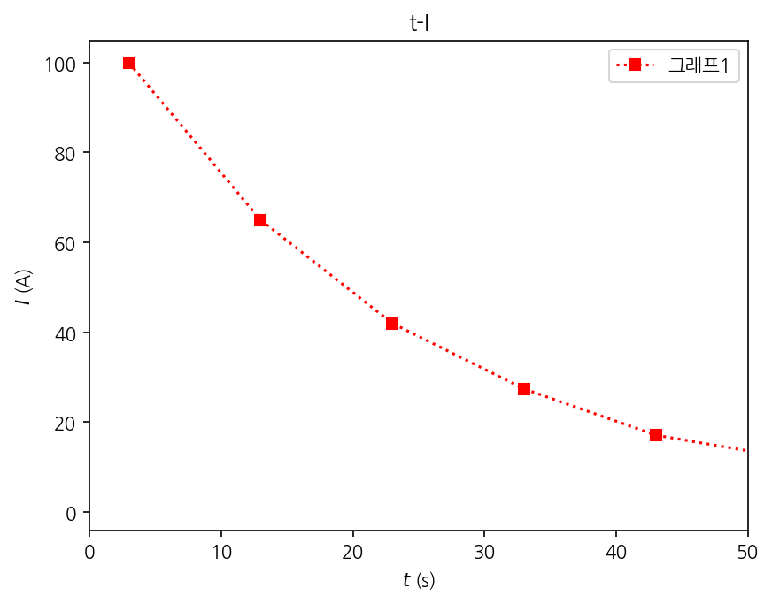
다음과 같이 color, marker, linestyle을 축약해서 지정할 수 있다.
plt.figure(dpi=150)
plt.title("t-I")
plt.xlabel("$t$ (s)")
plt.ylabel("$I$ (A)")
plt.plot(df["t"], df["I"], "rs:", label="그래프1") #이런방식도 가능, 이때 css 색상이나 헥스코드는 불가

plt.xlim(left=0, right=50)
plt.legend() #그래프 모두 그린 다음 입력해야 범례가 모두 표시됨
plt.show()
물론 다음과 같이 혼용해도 된다.
plt.figure(dpi=150)
plt.title("t-I")
plt.xlabel("$t$ (s)")
plt.ylabel("$I$ (A)")
plt.plot(df["t"], df["I"], "s--", label="그래프1", color="#388EDF") #이런방식도 가능

plt.xlim(left=0, right=50)
plt.legend() #그래프 모두 그린 다음 입력해야 범례가 모두 표시됨
plt.show()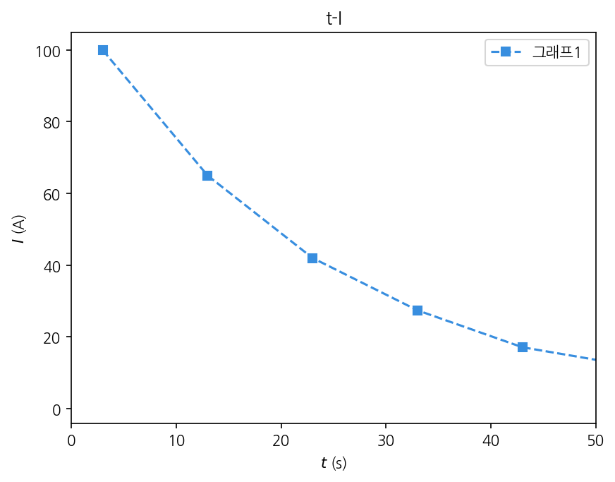
마커 종류나, 선 스타일, 다른 키워드 등은 공식 문서를 참고하면 된다.
https://matplotlib.org/stable/api/_as_gen/matplotlib.pyplot.plot.html
matplotlib.pyplot.plot — Matplotlib 3.8.2 documentation
An object with labelled data. If given, provide the label names to plot in x and y. Note Technically there's a slight ambiguity in calls where the second label is a valid fmt. plot('n', 'o', data=obj) could be plt(x, y) or plt(y, fmt). In such cases, the f
matplotlib.org
5.2 함수 그래프
점과 점사이의 간격을 좁게 하면 곡선으로 보이게 그릴 수 있다.
#함수 그래프
X = np.linspace(0, 3.141592*2, 100) #점의 간격을 촘촘하게 만들면 곡선처럼 보이게 그릴 수 있다.
Y = np.sin(X)

plt.figure(dpi=150)
plt.plot(X, Y)
plt.show()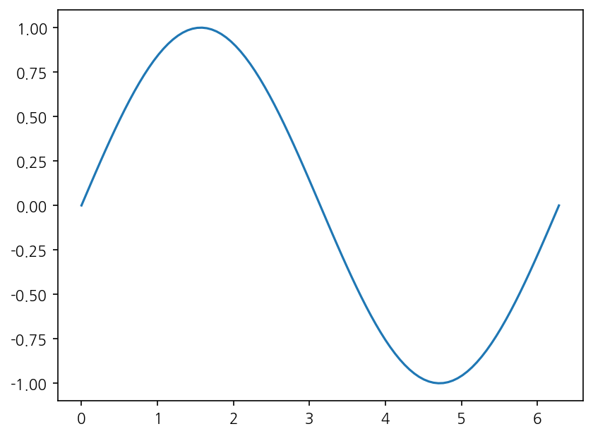
6.bar, barh, pie
#세로 막대 그래프 plt.bar()
month = ["apr", "may", "jun", "jul", "aug", "sep"]
sales = [1,2,3,5,2,1]
plt.title("month-sales")
plt.bar(month, sales, color='r')
plt.show()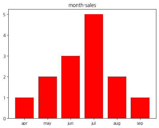
#가로 막대 그래프 plt.barh()
month = ["apr", "may", "jun", "jul", "aug", "sep"]
sales = [1,2,3,5,2,1]
plt.title("month-sales")
plt.barh(month, sales, color='y')
plt.show()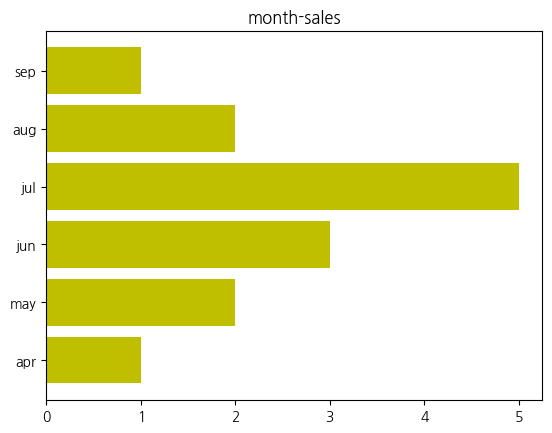
#그래프는 여러개를 같이 그릴 수 있다.
month = ["apr", "may", "jun", "jul", "aug", "sep"]
sales = [1,2,3,5,2,1]
plt.title("month-sales")
plt.bar(month, sales, color='g')
plt.plot(month, sales, color='r')
plt.show()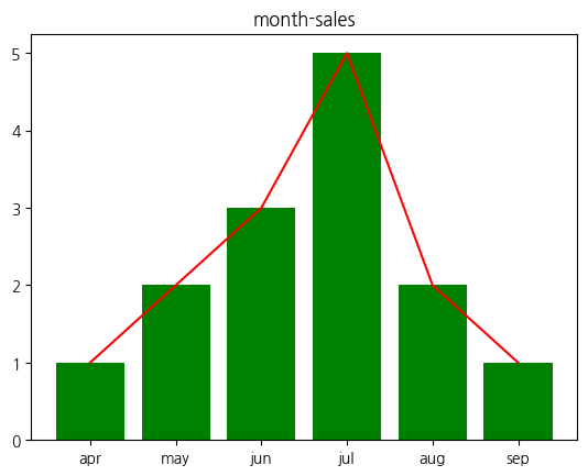
#파이 그래프
plt.title("혈액형")
blood_type = ['A', 'B', 'O', "AB"]
value = [26, 30, 20, 24]
plt.pie(value, labels=blood_type, autopct="%.1f%%") #autopct는 그래프 안 비율 표시 형식 지정
plt.show()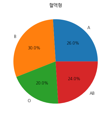
7.subplot -여러 그래프를 모아서 그리기
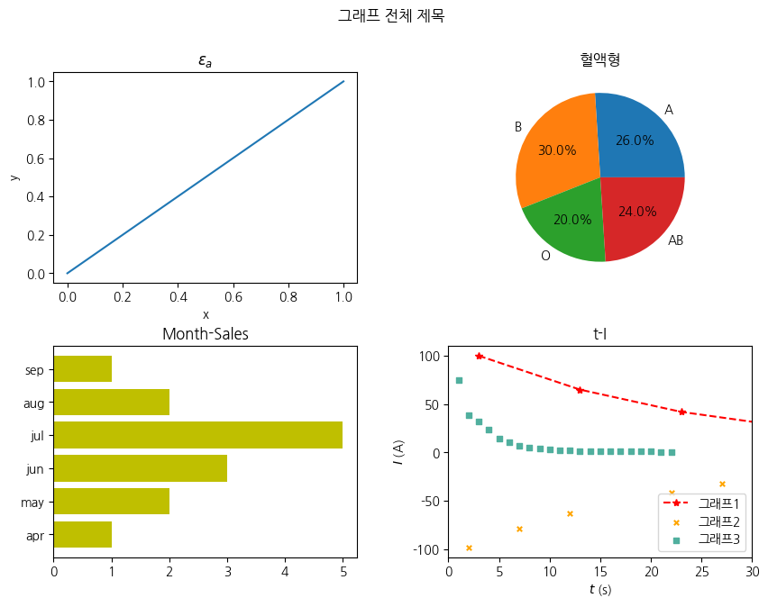
#subplot 여러 그래프 한번에 그리기
plt.figure()
fig, axes = plt.subplots(2, 2) #열 숫자, 행 숫자
fig.set_size_inches((10, 7)) #격자 크기 설정
plt.subplots_adjust(wspace=0.3, hspace=0.3) #격자간 여백 설정

fig.suptitle("그래프 전체 제목") #supxlabel, supylabel도 있음

#행, 열로 접근함, 행이 하나인 경우 axes[0], axes[1] 이렇게 접근해야하니 유의
axes[0,0].set_title("$\epsilon_a$") #키보드 ㅎ + 한자를 이용해 ε을 입력할 수도 있고, latex 문법을 이용해 그리스 문자를 입력할 수도 있다.
axes[0,0].plot([0,1], [0,1])
axes[0,0].set_xlabel('x')
axes[0,0].set_ylabel('y')

blood_type = ['A', 'B', 'O', "AB"]
value = [26, 30, 20, 24]
axes[0,1].set_title("혈액형")
axes[0,1].pie(value, labels=blood_type, autopct="%.1f%%")

month = ["apr", "may", "jun", "jul", "aug", "sep"]
sales = [1,2,3,5,2,1]
axes[1,0].set_title("Month-Sales")
axes[1,0].barh(month, sales, color='y')

axes[1,1].set_title("t-I")
axes[1,1].set_xlabel("$t$ (s)")
axes[1,1].set_ylabel("$I$ (A)")

axes[1,1].plot(df["t"], df["I"], label="그래프1", color='r', marker='*', ls="--")
axes[1,1].scatter(df2["t"], df2["I"], label="그래프2", s=15, color="orange", marker='x')
axes[1,1].scatter(df3["t"], df3["I"], label="그래프3", s=15, color="#50af9e", marker='s')

axes[1,1].set_xlim(left=0, right=30)
axes[1,1].legend() #그래프 모두 그린 다음 입력해야 범례가 모두 표시됨

fig.savefig("result.pdf", format="pdf", bbox_inches="tight")
8.projection="3d" -3차원 그래프 그리기
matplotlib 3.2.0 이후로 통합되어 Axes3D 등을 import할 필요가 없어졌다. 따라서 아래의 코드만으로 격자를 생성할 수 있다.
fig = plt.figure()
ax = fig.add_subplot(projection="3d")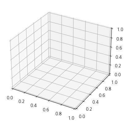
만약 여러개의 3d 격자를 생성하고 싶다면 일일히 add_subplot(projection="3d")이럴 필요 없이 아래 방법으로 할 수 있다.
fig, axes = plt.subplots(1, 3, figsize=(10, 3), subplot_kw={"projection":"3d"})
fig.suptitle("그래프 전체 제목")
fig.subplots_adjust(top=0.8) #doxgen comment를 잘 읽어볼 것

for i, ax in enumerate(axes):
    ax.set_title(f"title{i+1}")
    ax.set_xlabel(f"x{i+1}")
    ax.set_ylabel(f"y{i+1}")
    ax.set_zlabel(f"z{i+1}")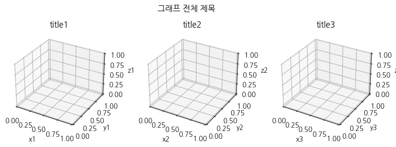
*이것저것 시도해보았으나 맨 오른쪽에 z축 라벨이 짤리는 것을 해결하지 못하였다.(방법을 아는 사람 알려주시면 감사하겠습니다.)
8.1 카메라 각도 조절
https://en.wikipedia.org/wiki/Azimuth 구면좌표계에서는 카메라의 Azimuthal angle(방위각)와 Elevation angle(앙각)이 있으며, 아래와 같이 설정할 수 있다.
fig = plt.figure()
ax = fig.add_subplot(projection="3d")
ax.view_init(elev=60, azim=10) #단위는 º(도, 60분법), azim 기본값 -45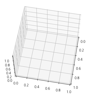
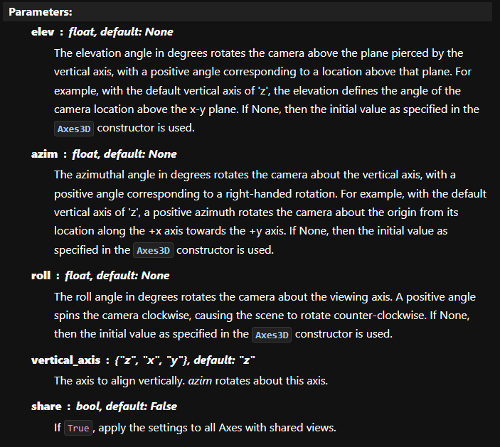
https://matplotlib.org/stable/api/_as_gen/mpl_toolkits.mplot3d.axes3d.Axes3D.view_init.html 추가적으로 roll을 지정하여 카메라 시선을 몇도 돌릴 것인지(+면 시계방향), 그리고 vertical_axis 옵션으로 Azimuthal angle의 기준이 될 수직 축을 지정할 수도 있다.(확대, 축소는 데이터 범위를 xlim, ylim으로 제한해서 보는 방법을 사용해야 한다.) eval=90는 꼭대기에서 내려다보는 것이며, azim=0은 x축이 카메라를 향하는 방향이다.
azim=0 
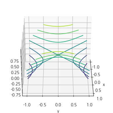
azim=10 위에서 내려다 보았을 때 기준으로 azim값이 양수면 시계방향으로 회전하는 것을 알 수 있다.
8.2 카메라 Angle Animation
#animation
fig = plt.figure()
ax = fig.add_subplot(projection="3d")

#from mpl_toolkits.mplot3d import Axes3D
from matplotlib import animation

def ani(i):
    ax.view_init(elev=40, azim=i)
    return fig, #, 안빠뜨리게 주의, 이부분 때문에 lambda 함수 사용 못함(사실 못하는건 아닌데 매우 지저분해짐)

anim = animation.FuncAnimation(fig, ani, frames=360, interval=20, blit=True) #interval은 프레임 사이 간격 (ms)
#blit은 blitting 여부
anim.save("3dani.gif", fps=30)
여기서 Blitting 옵션을 활성화하지 않으면, 프레임을 하나 만들때 마다 모든걸 그리지만, 활성화하면 움직이지 않는 배경은 그대로 두고 변하는 부분만 새로 그리기 때문에 애니메이션을 빠르게 만들 수 있게 해준다.
출처https://matplotlib.org/stable/users/explain/animations/blitting.html
Faster rendering by using blitting — Matplotlib 3.8.2 documentation
Faster rendering by using blitting Blitting is a standard technique in raster graphics that, in the context of Matplotlib, can be used to (drastically) improve performance of interactive figures. For example, the animation and widgets modules use blitting
matplotlib.org
참고로 2d 그래프에서도 animation 함수에 따라 아래와 같은 형태의 애니메이션도 가능하다.
from matplotlib import animation
import math
X = np.linspace(0, 2*math.pi, 100)
Y = np.sin(X)

fig = plt.figure()
ax = fig.add_subplot()
ax.set_xlim(left=0, right=2*math.pi)
ax.set_ylim(top=1.1, bottom=-1.1)

line, = plt.plot([], [])
def ani(i):
    line.set_data(X[:i], Y[:i])
    return line,

anim = animation.FuncAnimation(fig, ani, frames=100, interval=20, blit=True)
anim.save("2dani.gif", fps=30)
8.3 scatter(3D)
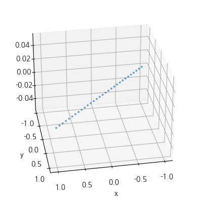
#scatter
X, Y = np.meshgrid(np.linspace(-1, 1, 30), np.linspace(-1, 1, 30))
fig = plt.figure()
ax = fig.add_subplot(projection="3d")
ax.set_xlabel("x")
ax.set_ylabel("y")
ax.view_init(azim=80)
ax.scatter(X, Y, X**2 - Y**2, alpha=0.5, s=4)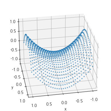
1차원의 배열을 2차원의 점들로 바꾸어 주는 것이 meshgrid 함수이다. 아래처럼 meshgrid를 사용하지 않으면, 3차원 직선에 불과하다. (정의역이 y=x (-1<x<1)에 위치하게 되니, x^2 - y^2 =0이 되기 때문이다.)
8.3 contour (등고선)
#contour
X, Y = np.meshgrid(np.linspace(-1, 1, 30), np.linspace(-1, 1, 30))
fig = plt.figure()
ax = fig.add_subplot(projection="3d")
ax.set_xlabel("x")
ax.set_ylabel("y")
ax.view_init(azim=80)
ax.contour(X, Y, X**2 - Y**2, levels=20) #levels 옵션으로 등고선 몇개 생성할 것인지 지정할 수 있다.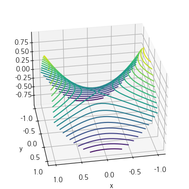
8.4 plot_wireframe
#plot_wireframe
X, Y = np.meshgrid(np.linspace(-1, 1, 30), np.linspace(-1, 1, 30))
fig = plt.figure()
ax = fig.add_subplot(projection="3d")
ax.set_xlabel("x")
ax.set_ylabel("y")
ax.view_init(azim=80)
ax.plot_wireframe(X, Y, X**2 - Y**2)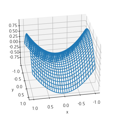
8.5 plot_surface
#plot_surface
X, Y = np.meshgrid(np.linspace(-1, 1, 30), np.linspace(-1, 1, 30))
fig = plt.figure()
ax = fig.add_subplot(projection="3d")
ax.set_xlabel("x")
ax.set_ylabel("y")
ax.view_init(azim=80)
ax.plot_surface(X, Y, X**2 - Y**2)
보기에 별로 좋지 않으니 colormap를 사용한 뒤 colorbar도 같이 표시해주자
#plot_surface
X, Y = np.meshgrid(np.linspace(-1, 1, 30), np.linspace(-1, 1, 30))
fig = plt.figure()
ax = fig.add_subplot(projection="3d")
ax.set_xlabel("x")
ax.set_ylabel("y")
ax.view_init(azim=80)
ax.plot_surface(X, Y, X**2 - Y**2, cmap="autumn")#cmap은 colormap
fig.colorbar(plt.autumn())
#컬러맵 종류 확인
plt.colormaps()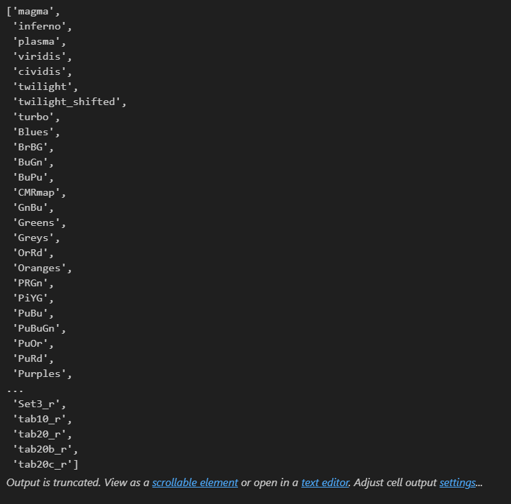
https://codetorial.net/matplotlib/set_colormap.html 8.6 plot_trisurf
앞에 plot_surface는 사각형 메쉬를 형성하였는데, 이 함수는 삼각형으로 메쉬를 형성한다. 삼각형 메쉬를 형성하기 위해선
점 3개씩 짝지어야 하므로 2차원 메쉬의 점들을 아래 코드 처럼 1차원으로 쭉나열해서 전달해주어야 한다.
#plot_trisurf
X, Y = np.meshgrid(np.linspace(-1, 1, 30), np.linspace(-1, 1, 30))
Z = X**2 - Y**2

fig = plt.figure()
ax = fig.add_subplot(projection="3d")
ax.set_xlabel("x")
ax.set_ylabel("y")
ax.view_init(azim=80)
ax.plot_trisurf(X.flatten(), Y.flatten(), Z.flatten(), cmap="autumn")
#ravel이나 reshape를 사용해도 결과는 같음
fig.colorbar(plt.autumn())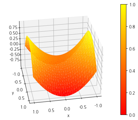
차근차근 과정을 살펴보자
먼저 meshgrid를 사용하면 아래처럼 출력 된다.
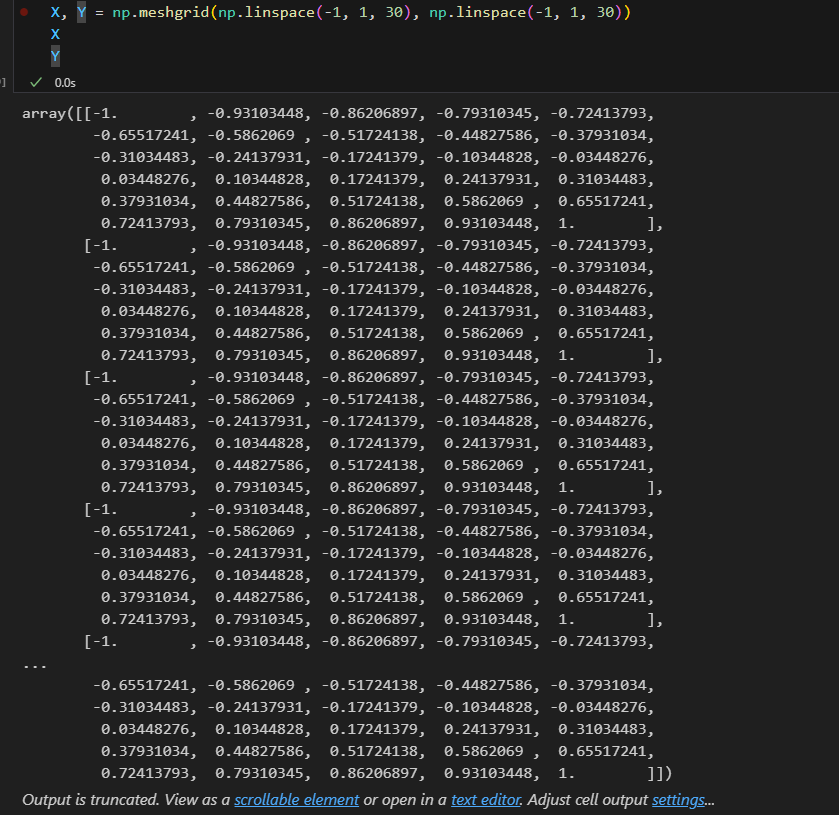
X 값 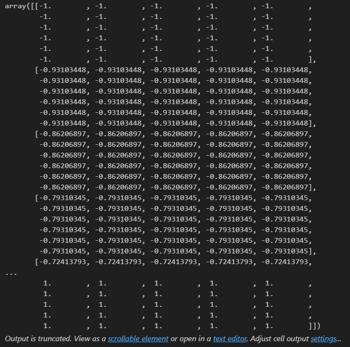
Y 값 사각형 영역을 가로로 슬라이스 한것을 알 수 있다.
다음으로 flatten, ravel, reshape을 살펴보자
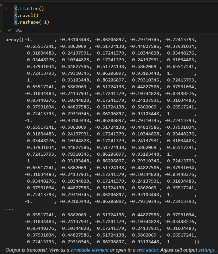
ravel 
reshape(-1) 모두 똑같이 2차원 배열을 꼬리 물기하듯 1차원으로 연결하였다.
참고로 당연히 다른 그래프와 같이 사용할 수 있다.
X, Y = np.meshgrid(np.linspace(-1, 1, 30), np.linspace(-1, 1, 30))
Z = X**2 - Y**2

fig = plt.figure()
ax = fig.add_subplot(projection="3d")
ax.set_xlabel("x")
ax.set_ylabel("y")
ax.view_init(azim=80)
ax.plot_trisurf(X.flatten(), Y.flatten(), Z.flatten(), cmap="autumn", alpha=0.7) #alpha 값은 투명도
ax.contour(X, Y, Z, levels=20, colors="k", linewidths=1)
fig.colorbar(plt.autumn())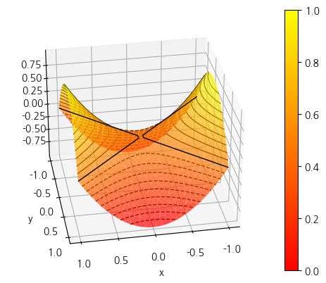
참고문헌
https://matplotlib.org/stable/api/index.html
API Reference — Matplotlib 3.8.2 documentation
axes: add data, limits, labels etc.
matplotlib.org
https://jehyunlee.github.io/2021/07/10/Python-DS-80-mpl3d2/
Matplotlib 3D Plots (2)
Matplotlib으로 3D Plot을 할 수 있습니다. 많은 분들이 알고 있는 사실이지만 적극적으로 쓰이지 않습니다. 막상 쓰려면 너무 낯설기도 하고 잘 모르기도 하기 때문입니다. Reference matplotlib tutorial: The
jehyunlee.github.io
2024.01.10 서문 추가
'파이썬 머신러닝' 카테고리의 다른 글
[재업]차원 축소와 주성분분석(Principal Component Anaylse, PCA) (1) 2024.02.09 머신러닝 가이드-지도학습 (0) 2023.07.02 파이썬 + VScode 머신러링 환경 구축 (0) 2023.07.02